Example: Benchmarking Isolation Forest with Probabilistic Outliers Prediction¶

Prerequisites¶

Python 3.12 (recommended)
Files on disk:
- database/train_dataset_severson.db (benchmark labels per cycle)
- database/train_features_severson.db (engineered features per cycle)
- PIPELINE_OUTPUT_DIR/hyperparams_iforest.csv (An example of tuned hyperparameters per cell for Isolation Forest)
(Optional) LaTeX installation if you want Matplotlib to render text with LaTeX:
- A TeX distribution (e.g., TeX Live/MacTeX/MiKTeX), dvipng, and fonts like cm-super.
- Don’t have LaTeX installed? Either install it, or set rcParams["text.usetex"] = False.

Before running the example in the quick_start_tutorials section, please evaluate whether the global directory path specified in src/osbad/config.py needs to be updated:

# Modify this global directory path if needed
PIPELINE_OUTPUT_DIR = Path.cwd().joinpath("artifacts_output_dir")

The following example of running a model with probabilistic outlier prediction is also provided as a notebook in quick_start_tutorials/02_run_model_tutorial.ipynb.

Step-1: Load libraries¶

Import the libraries into your local development environment, including the osbad library for benchmarking anomaly detection.

Path is used for robust, cross-platform file paths.
duckdb is the embedded analytical database engine storing the dataset.
fireducks.pandas as pd gives you a pandas-compatible API; you can usually treat it like import pandas as pd.
rcParams["text.usetex"] = True tells Matplotlib to render text via LaTeX. If you don’t have LaTeX installed, flip this to False.
bconf: project config utilities (e.g., where to write artifacts).
BenchDB: a thin layer around DuckDB that provides convenience loaders.
ModelRunner, hp, modval: modeling, hyperparameters, and model validation helpers for benchmarking study in this project.

# Standard library
import os
from pathlib import Path

# Third-party libraries
import duckdb
import fireducks.pandas as pd
import matplotlib.pyplot as plt
from matplotlib import rcParams

rcParams["text.usetex"] = True

# Custom osbad library for benchmarking anomaly detection
import osbad.config as bconf
import osbad.hyperparam as hp
import osbad.modval as modval
from osbad.database import BenchDB
from osbad.model import ModelRunner

Step-2: Load Benchmarking Dataset¶

Pick a specific cell based on the cell_index, which identifies the experimental data corresponding to one unique cell.
Create an artifacts folder for that cell, where you can save figures, tables, or model outputs related to this cell.
Initialize BenchDB for the selected cell and path to the DuckDB file: train_dataset_severson.db.
Loads all data related to selected_cell_label from the training partition.

# Get the cell-ID from unique_cell_index_train
selected_cell_label = "2017-05-12_5_4C-70per_3C_CH17"

# Create a subfolder to store fig output
# corresponding to each cell-index
selected_cell_artifacts_dir = bconf.artifacts_output_dir(
    selected_cell_label)

# Path to the DuckDB file:
# "train_dataset_severson.db"
db_filepath = (
    Path.cwd()
    .parent
    .joinpath("database","train_dataset_severson.db"))

# Import the BenchDB class
# Load only the dataset based on the selected cell
benchdb = BenchDB(
    db_filepath,
    selected_cell_label)

# load the benchmarking dataset
df_selected_cell = benchdb.load_benchmark_dataset(
    dataset_type="train")

Step-3: Load the Features DB¶

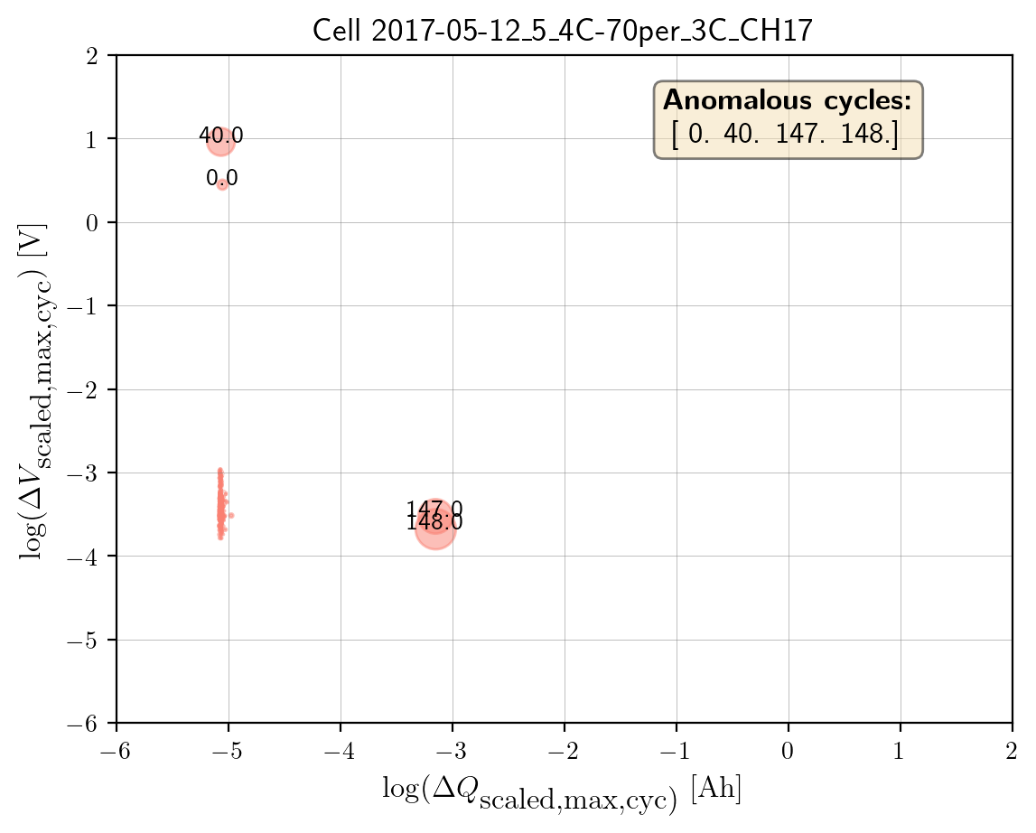
Load the features (e.g., log_max_diff_dQ, log_max_diff_dV) based on selected_cell_label in BenchDB.
To make the chart more informative, bubble sizes are scaled by ratios calculated from the distributions of feature values (max_diff_dQ and max_diff_dV). Using absolute values ensures all sizes are positive.
Plot the bubble chart using the logarithmic features log_max_diff_dQ and log_max_diff_dV as the x and y axes. Bubble sizes are determined by the calculated ratios. Cycles flagged as outliers are highlighted via their indices.

# Define the filepath to ``train_features_severson.db``
# DuckDB instance.
db_features_filepath = (
    Path.cwd()
    .parent
    .joinpath("database","train_features_severson.db"))

# Load only the training features dataset
df_features_per_cell = benchdb.load_features_db(
    db_features_filepath,
    dataset_type="train")

unique_cycle_count = (
    df_features_per_cell["cycle_index"].unique())

# Calculate the bubble size ratio for plotting
df_bubble_size_dQ = bstats.calculate_bubble_size_ratio(
    df_variable=df_features_per_cell["max_diff_dQ"])

df_bubble_size_dV = bstats.calculate_bubble_size_ratio(
    df_variable=df_features_per_cell["max_diff_dV"])

bubble_size = (
    np.abs(df_bubble_size_dV)
    * np.abs(df_bubble_size_dQ))

# Plot the bubble chart and label the outliers
axplot = bviz.plot_bubble_chart(
    xseries=df_features_per_cell["log_max_diff_dQ"],
    yseries=df_features_per_cell["log_max_diff_dV"],
    bubble_size=bubble_size,
    unique_cycle_count=unique_cycle_count,
    cycle_outlier_idx_label=true_outlier_cycle_index)

axplot.set_title(
    f"Cell {selected_cell_label}", fontsize=13)

axplot.set_xlabel(
    r"$\log(\Delta Q_\textrm{scaled,max,cyc)}\;\textrm{[Ah]}$",
    fontsize=12)
axplot.set_ylabel(
    r"$\log(\Delta V_\textrm{scaled,max,cyc})\;\textrm{[V]}$",
    fontsize=12)

output_fig_filename = (
    "log_bubble_plot_"
    + selected_cell_label
    + ".png")

fig_output_path = (
    selected_cell_artifacts_dir.joinpath(output_fig_filename))

plt.savefig(
    fig_output_path,
    dpi=200,
    bbox_inches="tight")

plt.show()

Bubble plot from ``2017-05-12_5_4C-70per_3C_CH17``

Step-4: Train model with tuned hyperparameters¶

Resolves PIPELINE_OUTPUT_DIR and reads hyperparams_iforest.csv and filters the CSV to the row for selected_cell_label.
Extracts the hyperparameter dictionary:
- contamination,
- n_estimators,
- max_samples,
- threshold.
Loads the Isolation Forest config from hp.MODEL_CONFIG["iforest"].
Builds a ModelRunner with the cell label, feature DataFrame, and selected features.
Calls runner.create_model_x_input() to get the X matrix (shape: n_cycles × n_features).
Instantiates the model with cfg.model_param(param_dict), fits it, and computes probabilities with predict_proba.
Converts probabilities into outlier indices and associated outlier scores.

# Access the global filepath variable PIPELINE_OUTPUT_DIR defined
# in config.py
PIPELINE_OUTPUT_DIR = bconf.PIPELINE_OUTPUT_DIR

# Read hyperparameters from the stored artifacts
hyperparam_filepath =  PIPELINE_OUTPUT_DIR.joinpath(
    "hyperparams_iforest.csv")
df_hyperparam_from_csv = pd.read_csv(hyperparam_filepath)

# Filter for the selected_cell_label
df_param_per_cell = df_hyperparam_from_csv[
    df_hyperparam_from_csv["cell_index"] == selected_cell_label]

# Hyperparameters for Isolation Forest
param_dict = {
    "contamination": df_param_per_cell["contamination"].values[0],
    "n_estimators": df_param_per_cell["n_estimators"].values[0],
    "max_samples": df_param_per_cell["max_samples"].values[0],
    "threshold": df_param_per_cell["threshold"].values[0]}


# Extract the model configuration for Isolation Forest
# Note: the dict key for Isolation Forest is iforest
cfg = hp.MODEL_CONFIG["iforest"]

# The two features implemented in this example
selected_feature_cols = (
    "log_max_diff_dQ",
    "log_max_diff_dV")

# Create a ModelRunner instance based on selected_cell_label,
# df_features_per_cell and
# selected_feature_cols
runner = ModelRunner(
    cell_label=selected_cell_label,
    df_input_features=df_features_per_cell,
    selected_feature_cols=selected_feature_cols
)

# Create the training input
Xdata = runner.create_model_x_input()

# Create the model based on the configured hyperparameters
model = cfg.model_param(param_dict)
print(model)

# Fit the model and get probabilistic outliers prediction
model.fit(Xdata)
proba = model.predict_proba(Xdata)

# Get the predicted outlier indices (pred_outlier_indices)
# pred_outlier_indices correspond to predicted anomalous cycles in the
# first example
(pred_outlier_indices,
 pred_outlier_score) = runner.pred_outlier_indices_from_proba(
    proba=proba,
    threshold=param_dict["threshold"],
    outlier_col=cfg.proba_col
)

Step-5: Predict Probabilistic Anomaly Score Map¶

pred_outlier_indices is a list of cycle indices predicted as anomalous by the Isolation Forest model. Using .isin(), we filter the dataframe to keep only the cycles identified as anomalies.
A new column, outlier_prob, is added to store the outliers probability computed by the model, making it easy to track how confidently the algorithm flags each cycle.
runner.predict_anomaly_score_map generates a 2D contour map of anomaly scores (outlier probability).

# Filter the selected features based on predicted outlier indices
df_outliers_pred = df_features_per_cell[
    df_features_per_cell["cycle_index"].isin(pred_outlier_indices)].copy()

df_outliers_pred["outlier_prob"] = pred_outlier_score

# Plot the anomaly score map
axplot = runner.predict_anomaly_score_map(
  selected_model=model,
  model_name="Isolation Forest",
  xoutliers=df_outliers_pred["log_max_diff_dQ"],
  youtliers=df_outliers_pred["log_max_diff_dV"],
  pred_outliers_index=pred_outlier_indices,
  threshold=param_dict["threshold"])

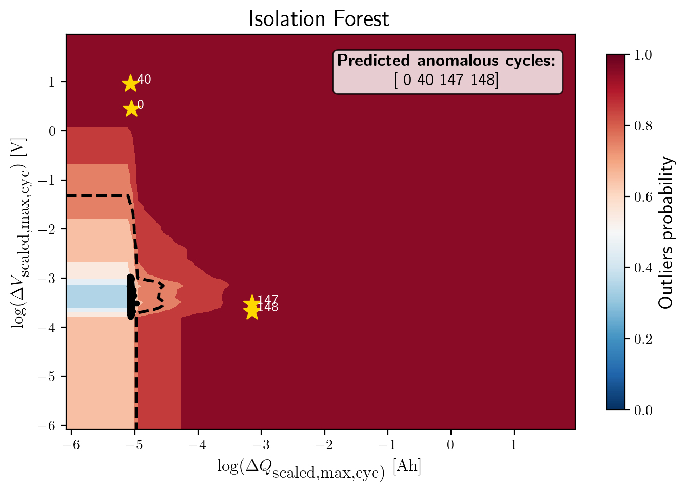
Anomaly score map with iForest from ``2017-05-12_5_4C-70per_3C_CH17``

The figure shows the anomaly score map produced by the Isolation Forest model:

Background Heatmap:
- Red regions: high anomaly probability (more likely to contain outliers).
- Blue/white regions: low anomaly probability (normal cycles).
Dashed Black Contour:
- Represents the decision boundary defined by the Isolation Forest threshold. Points outside are considered anomalies.
Black Dots:
- Represent the majority of normal cycles (inlier data).
Yellow Stars with Labels:
- Mark the detected anomalous cycles (0, 40, 147, 148).
- Their positions in the 2D feature space highlight where they deviate from typical battery behavior.
Colorbar (right):
- Quantifies anomaly probability (0 = normal, 1 = highly anomalous).
Annotation Box:
- Summarizes the predicted anomalous cycles.

Cycles 0 and 40 show unusually high voltage deviations, while 147 and 148 show strong deviations in charge capacity. These anomalies might correspond to specific battery degradation events, sensor errors, or experimental disturbances.

Step-6: Model performance evaluation¶

Map predicted outlier indices to the benchmark dataset:
- df_selected_cell holds cycle-level records and the ground-truth label (e.g., outlier = 1 for anomalous cycles, else 0).
- pred_outlier_indices is the list of cycle indices flagged by the model.
modval.evaluate_pred_outliers(...) returns a tidy DataFrame with:
- cycle_index: Cell discharge cycle index
- true_outlier: ground truth (0/1).
- pred_outlier: model prediction (0/1) for the same cycles.
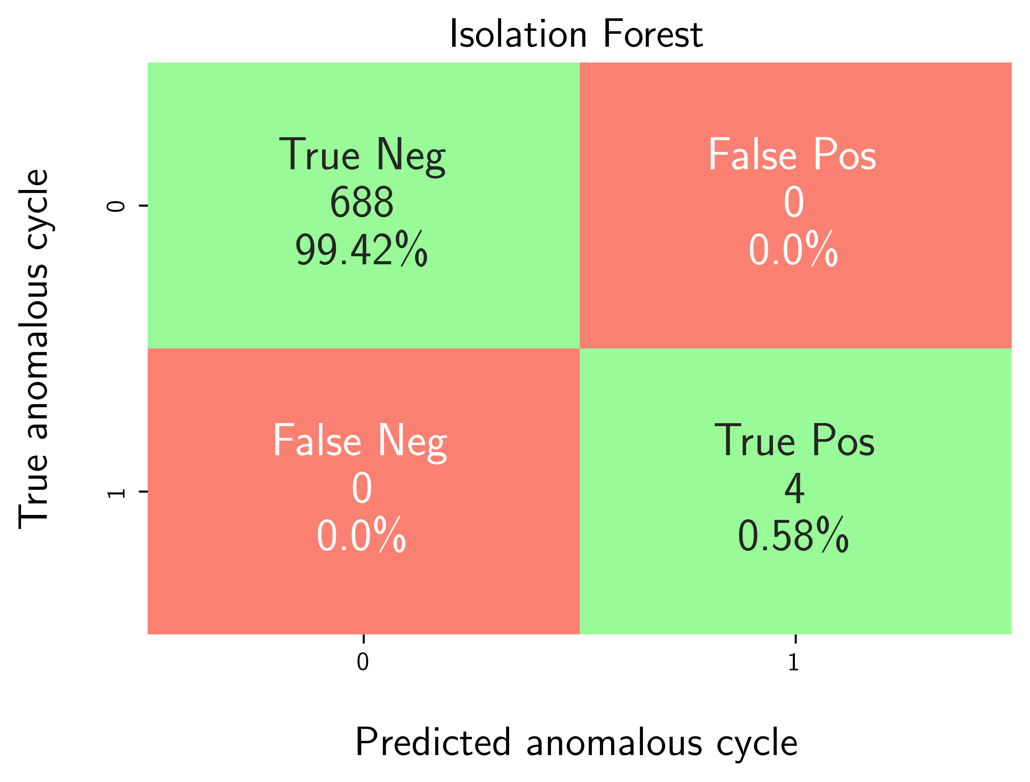
modval.generate_confusion_matrix(...) aggregates counts of:
- True Negative (TN): predicted 0, truth 0.
- False Positive (FP): predicted 1, truth 0.
- False Negative (FN): predicted 0, truth 1.
- True Positive (TP): predicted 1, truth 1.

# Map the predicted outlier indices
df_eval_outlier = modval.evaluate_pred_outliers(
  df_benchmark=df_selected_cell,
  outlier_cycle_index=pred_outlier_indices)

# Confusion matrix
axplot = modval.generate_confusion_matrix(
    y_true=df_eval_outlier["true_outlier"],
    y_pred=df_eval_outlier["pred_outlier"])

axplot.set_title(
    "Isolation Forest",
    fontsize=16)

output_fig_filename = (
    "conf_matrix_iforest_"
    + selected_cell_label
    + ".png")

fig_output_path = (
    selected_cell_artifacts_dir
    .joinpath(output_fig_filename))

plt.savefig(
    fig_output_path,
    dpi=600,
    bbox_inches="tight")

plt.show()

# Evaluate model performance
df_current_eval_metrics = modval.eval_model_performance(
    model_name="iforest",
    selected_cell_label=selected_cell_label,
    df_eval_outliers=df_eval_outlier)

Confusion matrix with iForest from ``2017-05-12_5_4C-70per_3C_CH17``