Example (4): Autoencoder with Hyperparameter Tuning (Tohoku Dataset)

Prerequisites

• Python 3.12 (recommended)

• Files on disk:

  • database/tohoku_benchmark_dataset.db (benchmark labels per cycle)

• (Optional) LaTeX installation if you want Matplotlib to render text with LaTeX:

  • A TeX distribution (e.g., TeX Live/MacTeX/MiKTeX), dvipng, and fonts like cm-super.

  • Don’t have LaTeX installed? Either install it, or set rcParams["text.usetex"] = False.

Before running the example in the machine_learning/hp_tuning_with_transfer_learning section, please evaluate whether the global directory path specified in src/osbad/config.py needs to be updated:

# Modify this global directory path if needed
PIPELINE_OUTPUT_DIR = Path.cwd().joinpath("artifacts_output_dir")

The following example of running an Autoencoder model with hyperparameter tuning is also provided as a notebook in machine_learning/hp_tuning_with_transfer_learning/tohoku_data_source/01_train_dataset/ml_06_autoencoder_hyperparam_tohoku.ipynb.

Step-1: Load libraries

Import the libraries into your local development environment, including the osbad library for benchmarking anomaly detection.

• Path is used for robust, cross-platform file paths.

• pprint pretty-prints data structures for readable diagnostics.

• duckdb is the embedded analytical database engine storing the dataset.

• optuna is a hyperparameter optimization framework used to search for the best model configuration.

• EmpiricalCovariance from scikit-learn is used to compute the Mahalanobis distance for feature engineering.

• bconf: project config utilities (e.g., where to write artifacts).

• hp: hyperparameter tuning utilities including the objective function, aggregation of best trials, and Pareto front visualization.

• BenchDB: a thin layer around DuckDB that provides convenience loaders.

• ModelRunner, modval, bviz: modeling, model validation, and visualization helpers for the benchmarking study.

# Standard library
from pathlib import Path
import pprint

# Third-party libraries
import duckdb
import pandas as pd
import matplotlib.pyplot as plt
import numpy as np
import optuna
from sklearn.covariance import EmpiricalCovariance

# Custom osbad library for anomaly detection
import osbad.config as bconf
import osbad.hyperparam as hp
import osbad.modval as modval
import osbad.viz as bviz
from osbad.database import BenchDB
from osbad.model import ModelRunner

Step-2: Load Benchmarking Dataset

• Define the path to the DuckDB database file (tohoku_benchmark_dataset.db) using the DB_DIR from bconf.

• Create a DuckDB connection (read-only) and load the full Tohoku dataset from the df_tohoku_dataset table.

• Drop the additional index column and retrieve the unique cell indices available in the dataset.

# Path to database directory
DB_DIR = bconf.DB_DIR

db_filepath = DB_DIR.joinpath("tohoku_benchmark_dataset.db")

# Create a DuckDB connection
con = duckdb.connect(
    db_filepath,
    read_only=True)

# Load all training dataset from duckdb
df_duckdb = con.execute(
    "SELECT * FROM df_tohoku_dataset").fetchdf()

# Drop the additional index column
df_duckdb = df_duckdb.drop(
    columns="__index_level_0__",
    errors="ignore")

unique_cell_index_train = df_duckdb["cell_index"].unique()
print(unique_cell_index_train)

Step-3: Filter Dataset for a Selected Cell

• There are 10 cells in the Tohoku dataset, and in this work, cell-1, cell-2, cell-5 and cell-6 are used for training.

• In this example, the model training is illustrated for one cell: cell_num_1.

• Pick a specific cell based on selected_cell_label, which identifies the experimental data corresponding to one unique cell.

• Create an artifacts folder for that cell, where you can save figures, tables, or model outputs related to this cell.

• Filter the loaded dataset for the selected cell only.

• Initialize BenchDB for the selected cell.

# Get the cell-ID from cell_inventory
selected_cell_label = "cell_num_1"
cell_num = selected_cell_label[-1]

# Create a subfolder to store fig output
# corresponding to each cell-index
selected_cell_artifacts_dir = bconf.artifacts_output_dir(
    selected_cell_label)

# Filter dataset for specific selected cell only
df_selected_cell = df_duckdb[
    df_duckdb["cell_index"] == selected_cell_label]

# Import the BenchDB class
benchdb = BenchDB(
    db_filepath,
    selected_cell_label)

Step-4: Drop True Labels

• Drop the true outlier labels (denoted as outlier) from the dataframe, keeping only the relevant columns for machine learning.

# Drop the outlier labels
df_selected_cell_without_labels = df_selected_cell.drop(
    "outlier", axis=1).reset_index(drop=True)

df_selected_cell_without_labels

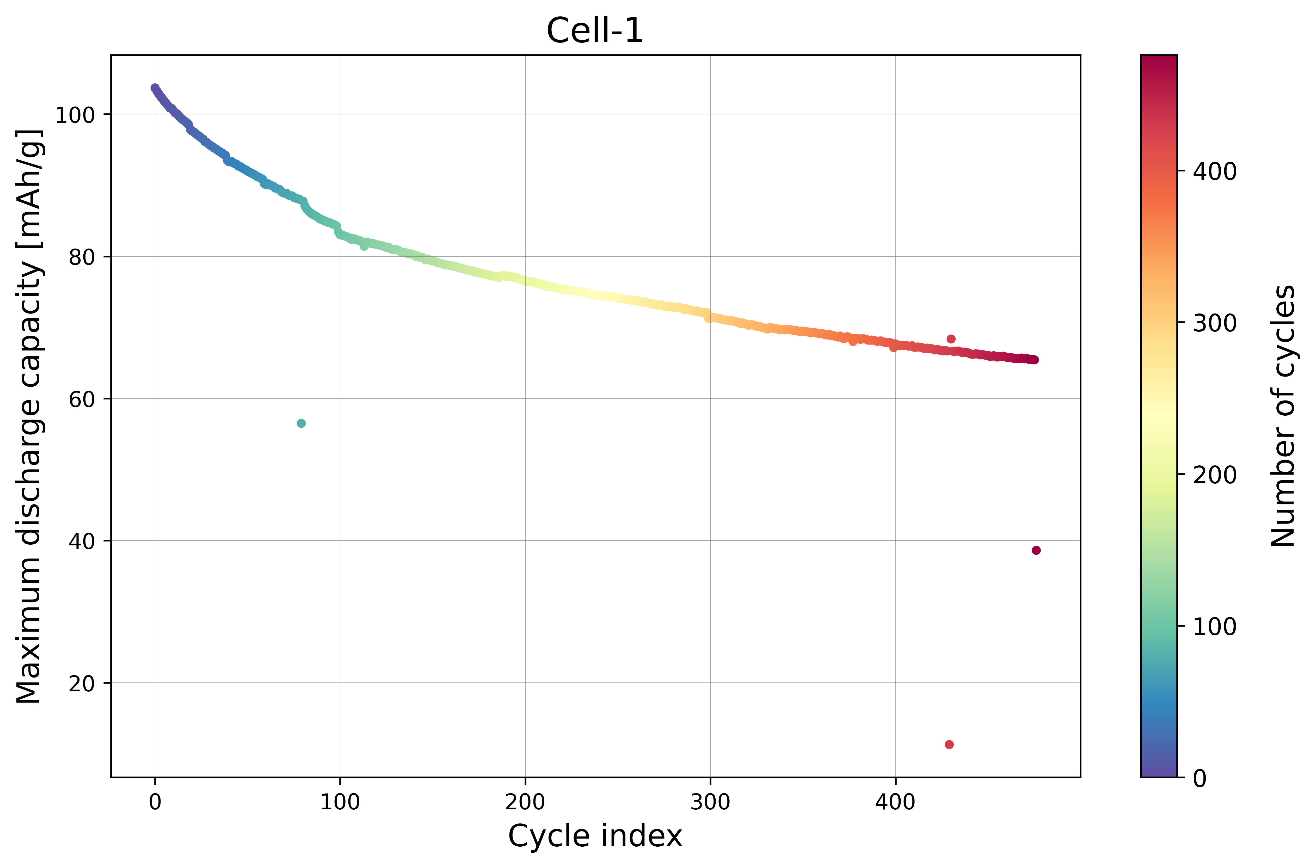
Step-5: Plot Cycle Capacity Fade without Labels

• Calculate the maximum discharge capacity per cycle.

• Visualize the capacity fade curve for the selected cell without displaying the true outlier labels. This represents what the model sees before training.

# Calculate maximum capacity per cycle
max_cap_per_cycle = (
    df_selected_cell_without_labels
        .groupby(["cycle_index"])["discharge_capacity"].max())
max_cap_per_cycle.name = "max_discharge_capacity"

unique_cycle_index = (
    df_selected_cell_without_labels["cycle_index"].unique())

axplot = bviz.plot_cycle_data(
    xseries=unique_cycle_index,
    yseries=max_cap_per_cycle,
    cycle_index_series=unique_cycle_index)

axplot.set_xlabel(
    r"Cycle index",
    fontsize=14)
axplot.set_ylabel(
    r"Maximum discharge capacity [mAh/g]",
    fontsize=14)

axplot.set_title(
    f"Cell-{cell_num}",
    fontsize=16)

output_fig_filename = (
    "cycling_data_without_labels_"
    + selected_cell_label
    + ".png")

fig_output_path = (
    selected_cell_artifacts_dir
    .joinpath(output_fig_filename))

plt.savefig(
    fig_output_path,
    dpi=600,
    bbox_inches="tight")

plt.show()

Step-6: Feature Transformation

In the Tohoku dataset, we want to track the sudden and unintended capacity drop over the cycle life. Therefore, the features used are:

• Cycle index: The cycle number of each cell.

• Maximum discharge capacity: Peak discharge capacity per cycle.

• Normalized Mahalanobis distance: A multivariate distance metric that accounts for the correlation between cycle index and maximum discharge capacity.

Create input features for Mahalanobis distance

The Mahalanobis distance is calculated from both the cycle index and the maximum discharge capacity.

df_cycle_index = pd.Series(
    unique_cycle_index,
    name="cycle_index")

# Input features for Mahalanobis distance
df_features_per_cell = pd.concat(
    [df_cycle_index,
     max_cap_per_cycle],
    axis=1)

df_features_per_cell

Compute the normalized Mahalanobis distance

• Fit an EmpiricalCovariance estimator to compute the covariance matrix of the feature space.

• Calculate the Mahalanobis distance for each cycle and normalize it by the maximum distance to obtain a value between 0 and 1.

Xfeat = df_features_per_cell.values

# Calculate Mahalanobis distance based on
# cycle_index and max_discharge_capacity
cov = EmpiricalCovariance().fit(Xfeat)
mahal_dist = cov.mahalanobis(Xfeat)

df_maha_dist = pd.Series(
    mahal_dist,
    name="mahal_dist")

# Merge calculated mahalanobis distance
df_merge_features = pd.concat(
    [df_features_per_cell,
     df_maha_dist], axis=1)

# Calculate maximum mahal_dist to
# normalize the distance calculation
max_mahal_dist = (
    df_merge_features["mahal_dist"].max())

df_merge_features["norm_mahal_dist"] = (
    df_merge_features["mahal_dist"]/max_mahal_dist)

selected_feature_cols = (
    "max_discharge_capacity",
    "norm_mahal_dist")

To inspect the merged features:

df_merge_features

Step-7: Hyperparameter Tuning with Optuna

Optuna is used to search for the best hyperparameters of the Autoencoder model. The multi-objective optimization maximizes both recall and precision simultaneously.

Define the hyperparameter search space

The hyperparameter search space is defined as a lambda function that maps each Optuna trial to a dictionary of sampled hyperparameter values:

• batch_size: Number of samples per training batch (int, 8 to 32).

• epoch_num: Number of training epochs (int, 10 to 50).

• learning_rate: Learning rate for the optimizer (float, 0.0 to 0.1).

• dropout_rate: Dropout rate for regularization (float, 0.1 to 0.5).

• threshold: Decision threshold for the outlier probability score (float, 0.0 to 1.0).

# Define the hyperparameter search space for autoencoder
hp_space=lambda trial: {
    "batch_size": trial.suggest_int(
        "batch_size", 8, 32),
    "epoch_num": trial.suggest_int(
        "epoch_num", 10, 50),
    "learning_rate": trial.suggest_float(
        "learning_rate", 0.0, 0.1),
    "dropout_rate": trial.suggest_float(
        "dropout_rate", 0.1, 0.5),
    "threshold": trial.suggest_float(
        "threshold", 0.0, 1.0)}

Create and run the Optuna study

• A TPESampler with a fixed seed ensures reproducibility.

• The study is configured for multi-objective optimization with two directions set to maximize (recall and precision).

• The hp.objective function trains the Autoencoder model for each trial and evaluates it against the benchmarking dataset.

# Instantiate an optuna study for autoencoder model
sampler = optuna.samplers.TPESampler(seed=42)

autoencoder_study = optuna.create_study(
    study_name="autoencoder_hyperparam",
    sampler=sampler,
    directions=["maximize","maximize"])

autoencoder_study.optimize(
    lambda trial: hp.objective(
        trial,
        model_id="autoencoder",
        df_feature_dataset=df_merge_features,
        selected_feature_cols=selected_feature_cols,
        df_benchmark_dataset=df_selected_cell,
        hp_space=hp_space,
        selected_cell_label=selected_cell_label),
    n_trials=20)

Step-8: Aggregate Best Trials

After the optimization completes, aggregate the best trial hyperparameters using the median (or median rounded to integer for discrete parameters). The aggregation schema defines how each hyperparameter is consolidated across the Pareto-optimal trials:

schema_autoencoder = {
    "batch_size": "median_int",
    "epoch_num": "median_int",
    "learning_rate": "median",
    "dropout_rate": "median",
    "threshold": "median",
}

df_autoencoder_hyperparam = hp.aggregate_best_trials(
    autoencoder_study.best_trials,
    cell_label=selected_cell_label,
    model_id="autoencoder",
    schema=schema_autoencoder)

df_autoencoder_hyperparam

Step-9: Evaluate Percentage of Perfect Recall and Precision

• Evaluate the percentage of trials in the study that achieved a perfect recall score (= 1.0) and a perfect precision score (= 1.0).

• This provides insight into how frequently the optimization found configurations that correctly identified all anomalies without any false positives.

recall_score_pct, precision_score_pct = hp.evaluate_hp_perfect_score_pct(
    model_study=autoencoder_study)

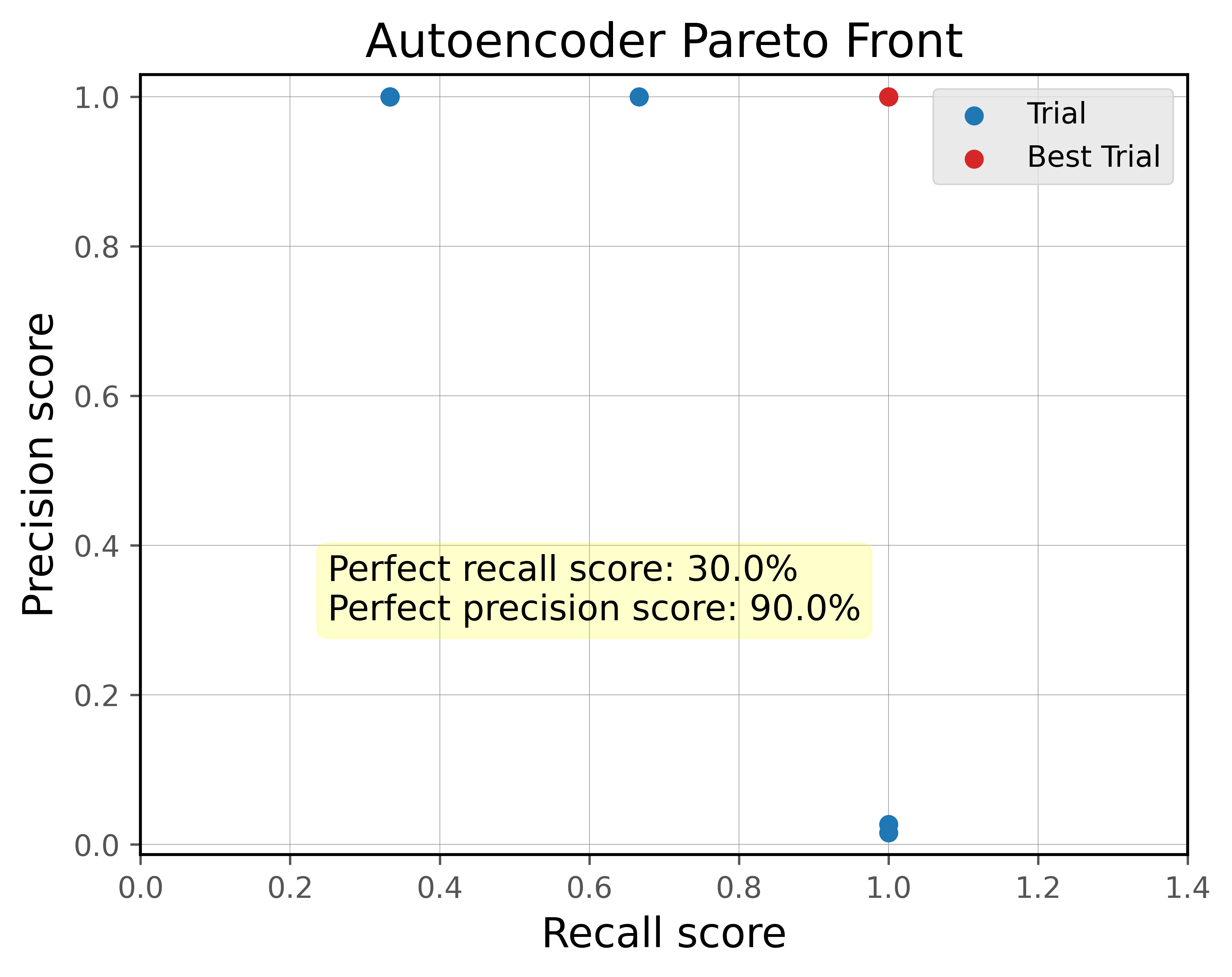
Step-10: Plot Pareto Front

• The Pareto front visualizes the trade-off between recall and precision across all trials.

• Trials on the Pareto front represent the best achievable combinations of recall and precision: improving one metric would require sacrificing the other.

hp.plot_pareto_front(
    autoencoder_study,
    selected_cell_label,
    fig_title="Autoencoder Pareto Front")

plt.show()

Step-11: Export Hyperparameters to CSV

• Export the aggregated best hyperparameters to a CSV file for record-keeping and reproducibility.

• The if_exists="replace" option overwrites any existing entry for the selected cell.

# Export current hyperparameters to CSV
hyperparam_filepath =  Path.cwd().joinpath(
    "hp_06_autoencoder_hyperparam_tohoku.csv")

hp.export_current_hyperparam(
    df_autoencoder_hyperparam,
    selected_cell_label,
    export_csv_filepath=hyperparam_filepath,
    if_exists="replace")

Step-12: Train Model with Best Trial Parameters

Load best trial parameters from CSV output

• Read back the exported hyperparameters from CSV and filter for the selected cell.

# Test reading from exported metrics
df_hyperparam_from_csv = pd.read_csv(hyperparam_filepath)

df_param_per_cell = df_hyperparam_from_csv[
    df_hyperparam_from_csv["cell_index"] == selected_cell_label]
df_param_per_cell

Create a dict for best trial parameters

param_dict = df_param_per_cell.iloc[0].to_dict()
pprint.pp(param_dict)

Run the model with best trial parameters

• Extract the model configuration for the Autoencoder from hp.MODEL_CONFIG.

• Instantiate a ModelRunner with the selected features and cell label.

• Build the training input matrix Xdata (shape: n_cycles × n_features).

• Create the Autoencoder model using the tuned hyperparameters via cfg.model_param(param_dict).

• Fit the model, compute probabilistic outlier scores, and extract the predicted outlier cycle indices using the tuned threshold.

cfg = hp.MODEL_CONFIG["autoencoder"]

runner = ModelRunner(
    cell_label=selected_cell_label,
    df_input_features=df_merge_features,
    selected_feature_cols=selected_feature_cols
)

Xdata = runner.create_model_x_input()

model = cfg.model_param(param_dict)
print(model)
model.fit(Xdata)
proba = model.predict_proba(Xdata)

pred_outlier_indices, pred_outlier_score = runner.pred_outlier_indices_from_proba(
    proba=proba,
    threshold=param_dict["threshold"],
    outlier_col=cfg.proba_col
)

pred_outlier_indices, pred_outlier_score

Get predicted outlier dataframe

• Filter the feature dataframe to retain only cycles predicted as anomalous.

• Append the outlier_prob column with the model’s outlier probability for each predicted anomalous cycle.

df_outliers_pred = (df_merge_features[
    df_merge_features["cycle_index"]
    .isin(pred_outlier_indices)].copy())

df_outliers_pred["outlier_prob"] = pred_outlier_score
df_outliers_pred

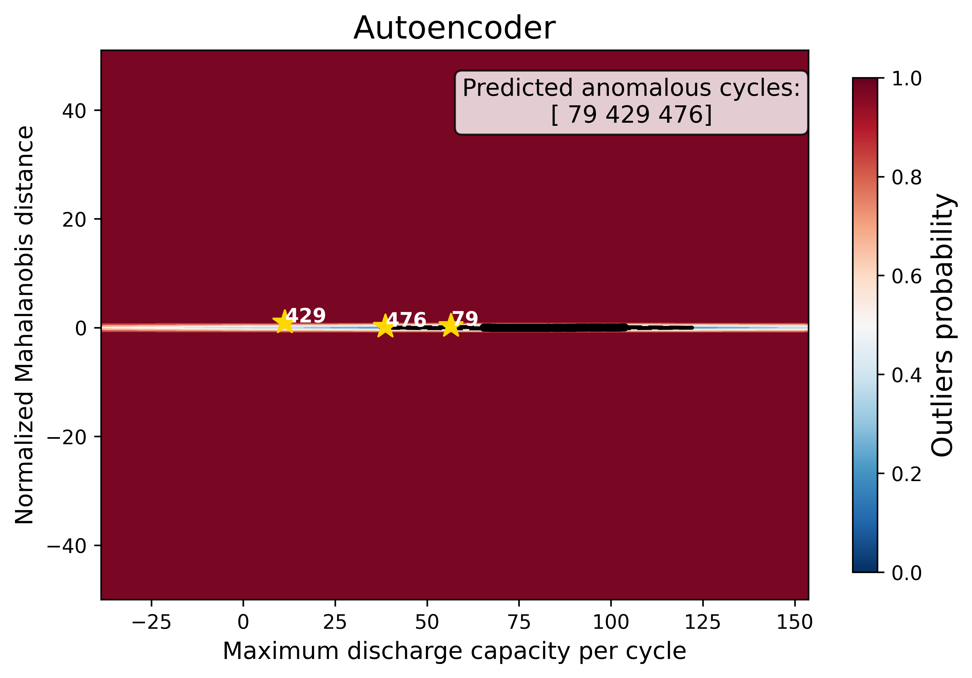
Step-13: Predict Probabilistic Anomaly Score Map

• runner.predict_anomaly_score_map generates a 2D contour map of anomaly scores (outlier probability).

• The anomaly score map uses the tuned threshold from the hyperparameter optimization.

• Two different grid_offset values are shown to demonstrate how the grid resolution affects the visualization.

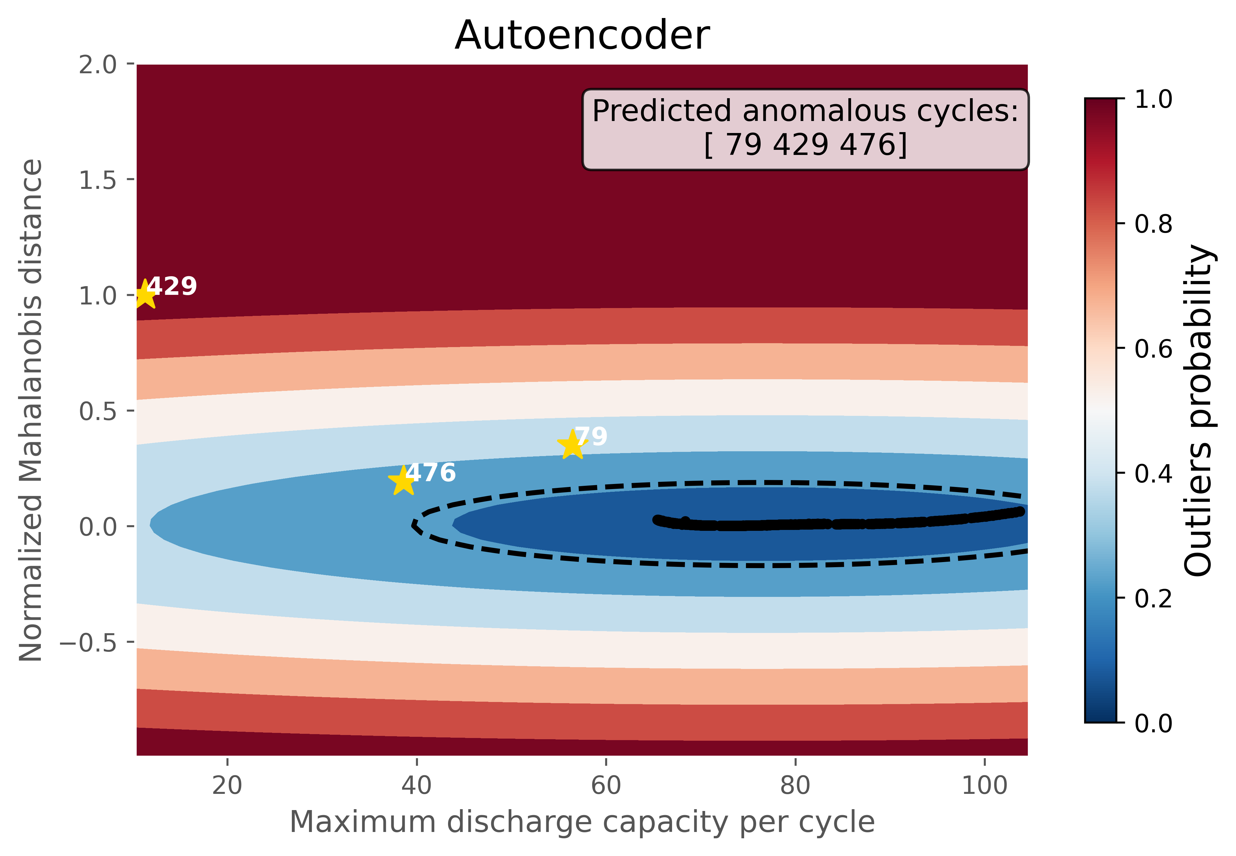
Anomaly score map with grid offset = 1

grid_offset_size = 1

axplot = runner.predict_anomaly_score_map(
    selected_model=model,
    model_name="Autoencoder",
    xoutliers=df_outliers_pred["max_discharge_capacity"],
    youtliers=df_outliers_pred["norm_mahal_dist"],
    pred_outliers_index=pred_outlier_indices,
    threshold=param_dict["threshold"],
    square_grid=False,
    grid_offset=grid_offset_size
)

axplot.set_xlabel(
    r"Maximum discharge capacity per cycle",
    fontsize=12)
axplot.set_ylabel(
    r"Normalized Mahalanobis distance",
    fontsize=12)

output_fig_filename = (
    f"autoencoder_grid_offset_size_{grid_offset_size}_"
    + selected_cell_label
    + ".png")

fig_output_path = (
    selected_cell_artifacts_dir
    .joinpath(output_fig_filename))

plt.savefig(
    fig_output_path,
    dpi=600,
    bbox_inches="tight")

plt.show()

Anomaly score map with grid offset = 50

grid_offset_size = 50

axplot = runner.predict_anomaly_score_map(
    selected_model=model,
    model_name="Autoencoder",
    xoutliers=df_outliers_pred["max_discharge_capacity"],
    youtliers=df_outliers_pred["norm_mahal_dist"],
    pred_outliers_index=pred_outlier_indices,
    threshold=param_dict["threshold"],
    square_grid=False,
    grid_offset=grid_offset_size
)

axplot.set_xlabel(
    r"Maximum discharge capacity per cycle",
    fontsize=12)
axplot.set_ylabel(
    r"Normalized Mahalanobis distance",
    fontsize=12)

output_fig_filename = (
    f"autoencoder_grid_offset_size_{grid_offset_size}_"
    + selected_cell_label
    + ".png")

fig_output_path = (
    selected_cell_artifacts_dir
    .joinpath(output_fig_filename))

plt.savefig(
    fig_output_path,
    dpi=600,
    bbox_inches="tight")

plt.show()

The figure shows the anomaly score map produced by the hyperparameter-tuned Autoencoder model:

• Background Heatmap:

  • Red regions: high anomaly probability (more likely to contain outliers).

  • Blue/white regions: low anomaly probability (normal cycles).

• Dashed Black Contour:

  • Represents the decision boundary defined by the optimized threshold. Points outside are considered anomalies.

• Black Dots:

  • Represent the majority of normal cycles (inlier data).

• Yellow Stars with Labels:

  • Mark the detected anomalous cycles. Their positions in the 2D feature space highlight where they deviate from typical battery behavior.

• Colorbar (right):

  • Quantifies anomaly probability (0 = normal, 1 = highly anomalous).

Step-14: Model Performance Evaluation

• Map predicted outlier indices to the benchmark dataset to compare against ground-truth labels.

• modval.evaluate_pred_outliers(...) returns a tidy DataFrame with:

  • cycle_index: Cell discharge cycle index.

  • true_outlier: ground truth (0/1).

  • pred_outlier: model prediction (0/1) for the same cycles.

df_eval_outlier = modval.evaluate_pred_outliers(
    df_benchmark=df_selected_cell,
    outlier_cycle_index=pred_outlier_indices)

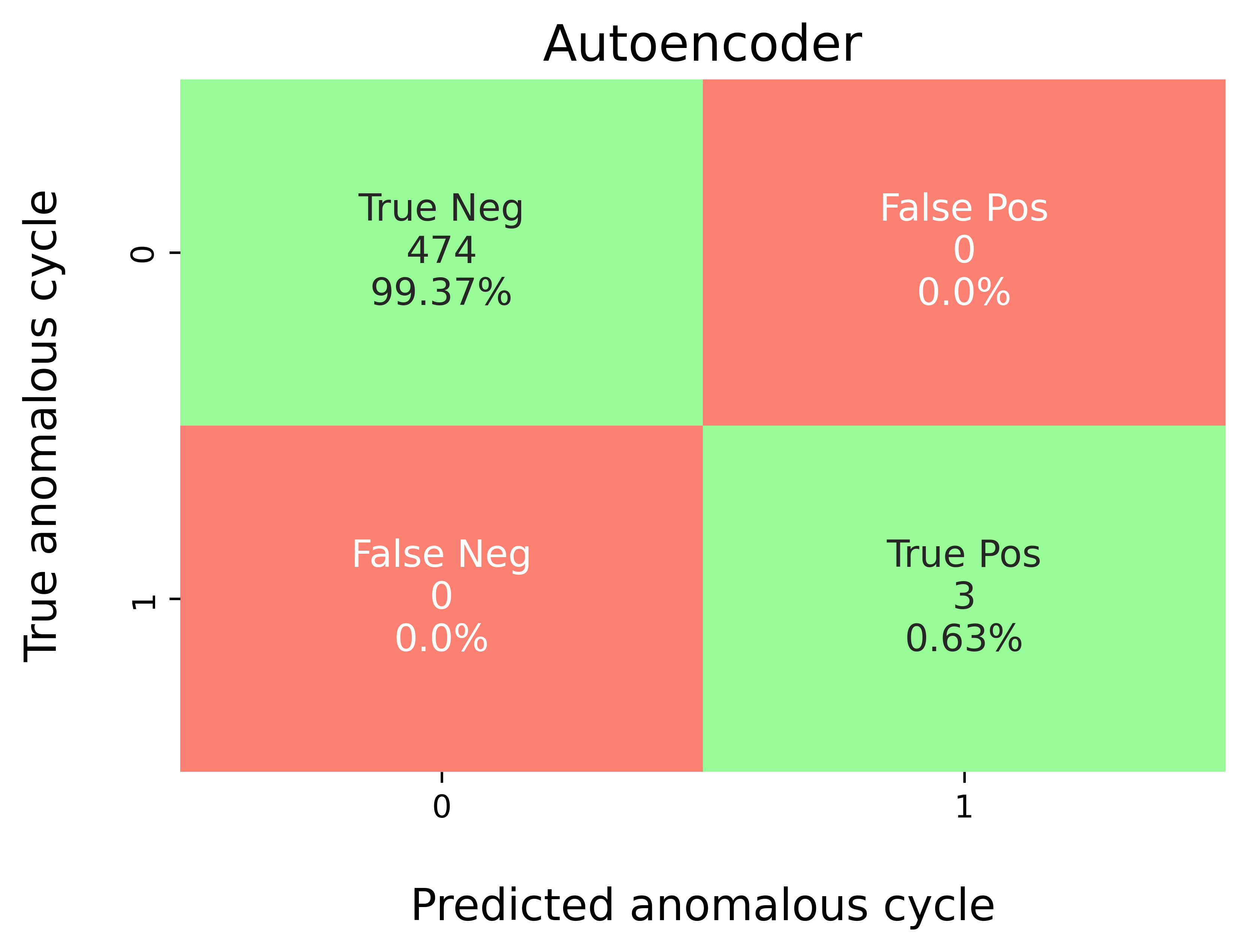
Confusion matrix

axplot = modval.generate_confusion_matrix(
    y_true=df_eval_outlier["true_outlier"],
    y_pred=df_eval_outlier["pred_outlier"])

axplot.set_title(
    "Autoencoder",
    fontsize=16)

output_fig_filename = (
    "conf_matrix_autoencoder_"
    + selected_cell_label
    + ".png")

fig_output_path = (
    selected_cell_artifacts_dir
    .joinpath(output_fig_filename))

plt.savefig(
    fig_output_path,
    dpi=600,
    bbox_inches="tight")

plt.show()

Evaluation metrics

In this study, five different metrics are used to evaluate model performance:

• Accuracy: \(\frac{\textrm{TP} + \textrm{TN}}{\textrm{Total prediction}}\)

• Precision: \(\frac{\textrm{TP}}{\textrm{TP + FP}}\)

• Recall: \(\frac{\textrm{TP}}{\textrm{TP + FN}}\)

• F1-score: \(\frac{2(\textrm{Precision}\times \textrm{Recall})}{\textrm{Precision} + \textrm{Recall}}\)

• MCC: \(\frac{TP \times TN - FP \times FN}{\sqrt{(TP + FP)(TP + FN)(TN + FP)(TN+FN)}}\)

df_current_eval_metrics = modval.eval_model_performance(
    model_name="autoencoder",
    selected_cell_label=selected_cell_label,
    df_eval_outliers=df_eval_outlier)

df_current_eval_metrics

Step-15: Export Model Performance Metrics

• Export the evaluation metrics to a CSV file for record-keeping and comparison across models and cells.

# Export current metrics to CSV
hyperparam_eval_filepath =  Path.cwd().joinpath(
    "eval_metrics_hp_single_cell_tohoku.csv")

hp.export_current_model_metrics(
    model_name="autoencoder",
    selected_cell_label=selected_cell_label,
    df_current_eval_metrics=df_current_eval_metrics,
    export_csv_filepath=hyperparam_eval_filepath,
    if_exists="replace")

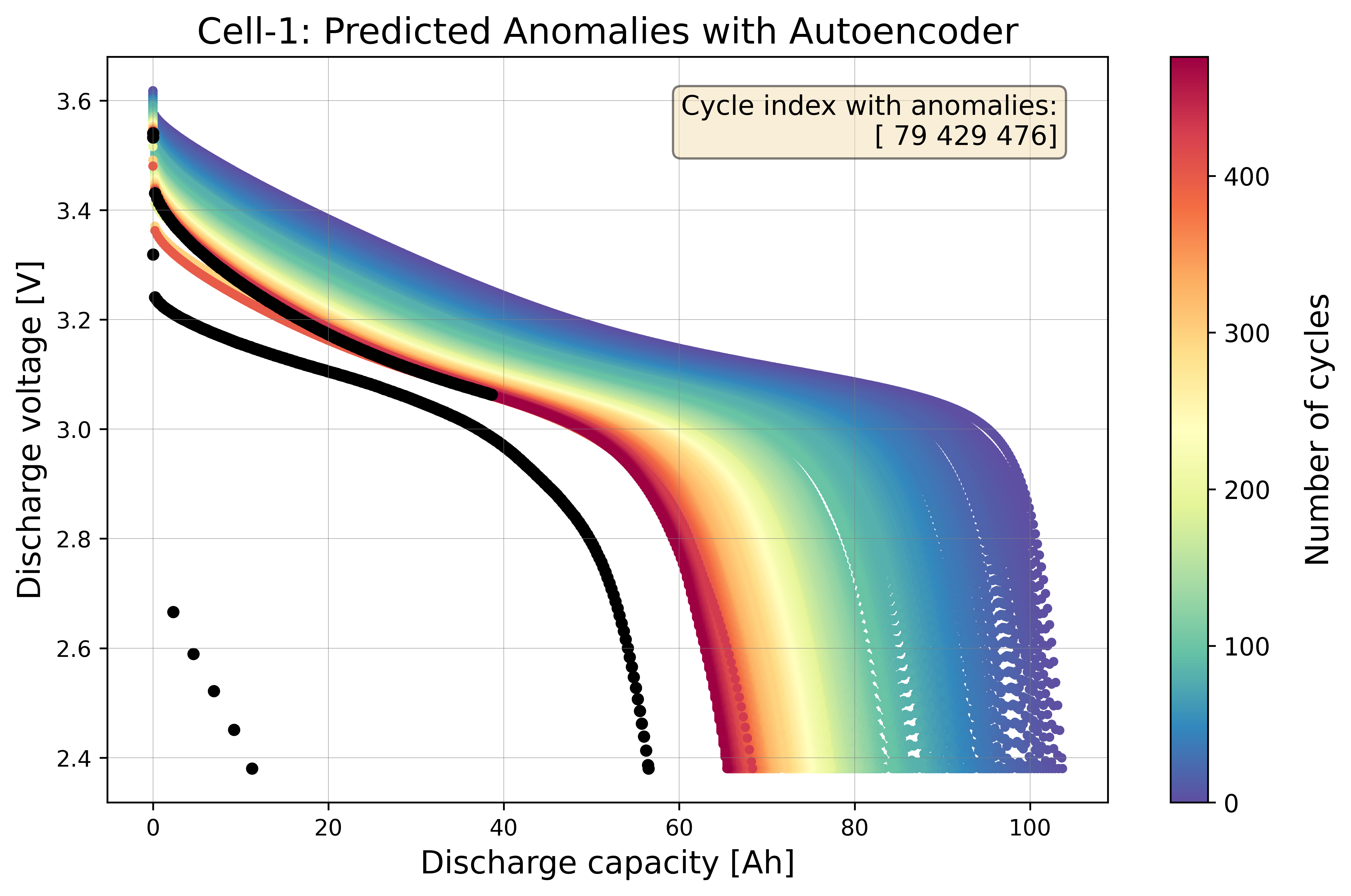
Step-16: Visualize Predicted Anomalies

Plot predicted anomalous cycles

• Re-plot the cycling data with the predicted anomalous cycles highlighted and annotated, allowing visual comparison of model predictions against the ground truth.

axplot = benchdb.plot_cycle_data(
    df_selected_cell_without_labels,
    pred_outlier_indices)

axplot.set_title(
    f"Cell-{cell_num}: Predicted Anomalies with Autoencoder",
    fontsize=16)

output_fig_filename = (
    "autoencoder_pred_cycles_with_outliers_"
    + selected_cell_label
    + ".png")

fig_output_path = (
    selected_cell_artifacts_dir
    .joinpath(output_fig_filename))

plt.savefig(
    fig_output_path,
    dpi=600,
    bbox_inches="tight")

plt.show()

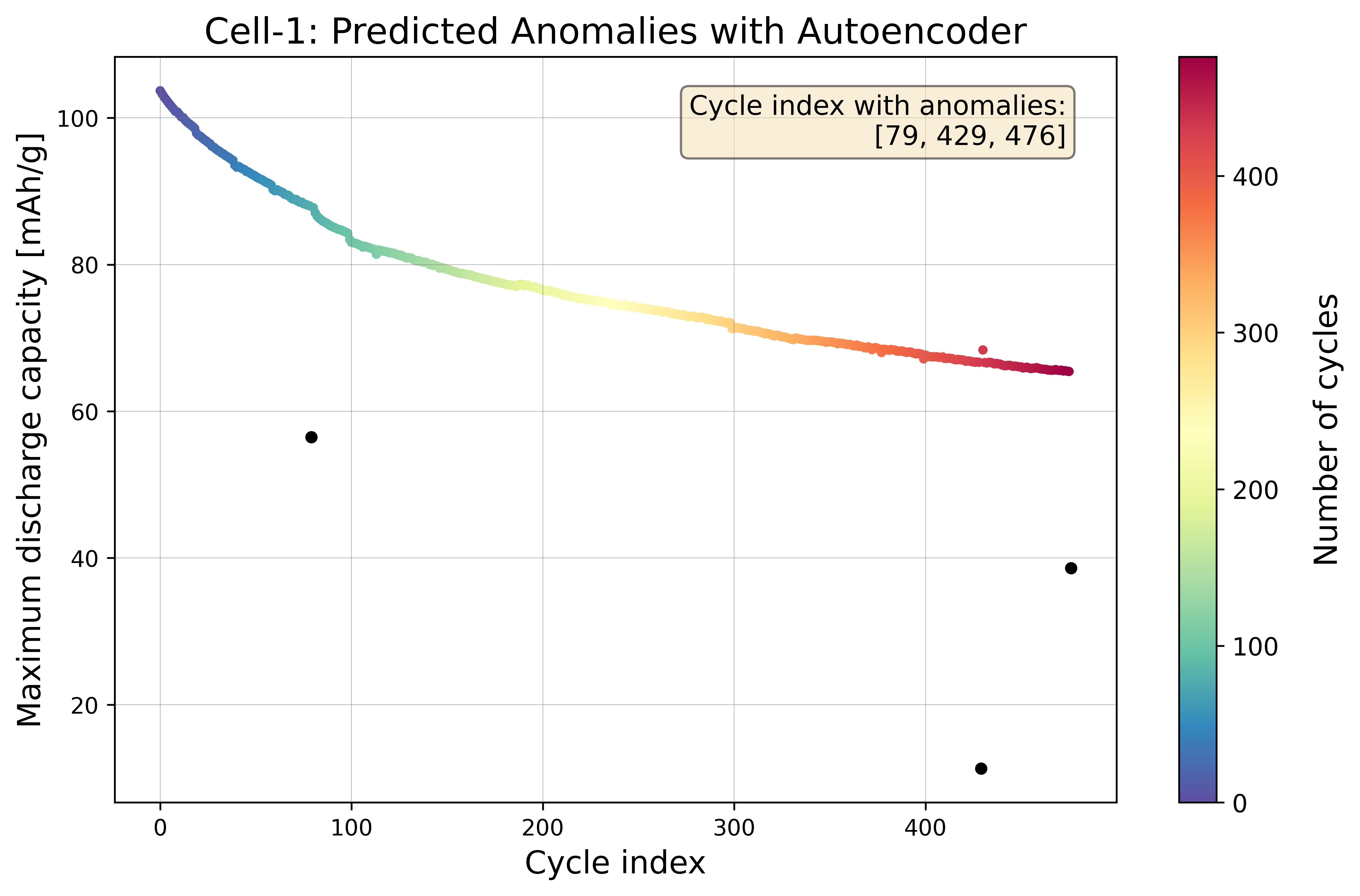
Plot predicted capacity fade with outlier annotations

• Filter the maximum capacity per cycle to retain only the predicted outlier cycles.

• Plot the capacity fade curve with the predicted outlier cycles annotated in a text box.

pred_cap_outlier = max_cap_per_cycle[
    max_cap_per_cycle
        .index.isin(pred_outlier_indices)]

axplot = bviz.plot_cycle_data(
    xseries=unique_cycle_index,
    yseries=max_cap_per_cycle,
    cycle_index_series=unique_cycle_index,
    xoutlier=pred_cap_outlier.index,
    youtlier=pred_cap_outlier)

axplot.set_xlabel(
    r"Cycle index",
    fontsize=14)
axplot.set_ylabel(
    r"Maximum discharge capacity [mAh/g]",
    fontsize=14)

axplot.set_title(
    f"Cell-{cell_num}: Predicted Anomalies with Autoencoder",
    fontsize=16)

# Create textbox to annotate anomalous cycle
textstr = '\n'.join((
    r"Cycle index with anomalies:",
    f"{list(pred_cap_outlier.index)}"))

# properties for bbox
props = dict(
    boxstyle='round',
    facecolor='wheat',
    alpha=0.5)

axplot.text(
    0.95, 0.95,
    textstr,
    transform=axplot.transAxes,
    fontsize=12,
    ha="right", va='top',
    bbox=props)

output_fig_filename = (
    "autoencoder_pred_cap_fade_with_outliers_"
    + selected_cell_label
    + ".png")

fig_output_path = (
    selected_cell_artifacts_dir
    .joinpath(output_fig_filename))

plt.savefig(
    fig_output_path,
    dpi=600,
    bbox_inches="tight")

plt.show()

---

Note

This notebook serves as an example to explain the workflow for running the Autoencoder model with hyperparameter tuning on a single cell. To mitigate overfitting, the model should be trained and validated across multiple cells in the training dataset instead of a single cell.

The hyperparameters are then averaged across all cells to find a more generalizable configuration that performs well across the entire dataset, rather than just one cell.